Example Interactomcis usecase for ProteoGyver

This guide documents the end to end QC analysis of a public interactomics dataset.

Software and data prerequisites

For this example, we used a publicly available dataset (MSV000095163, Original paper)

Since the goal is not to demo how to use FragPipe, default workflows will be used, with minimal consideration given to e.g. parameters of different mass spectrometers. As long as the library used is from the same organism, we will identify enough proteins to demo PG. In a real use scenario, parameters in MSFragger in particular should be set according to the MS settings. For this reason, default FragPipe workflow was used with a recent Human fasta proteome downloaded from UniProt. To save time on searches, only a subset of 30 runs were analyzed (see sample table below)

Proteogyver

This example assumes you have proteogyver running in a docker container already. If not, refer to the main readme file for install instructions.

Data upload

For data upload, the combined_protein.tsv from the FragPipe output was used as the data table, and for sample table, a tsv file with the following contents was created:

Sample name	Sample group	Bait uniprot
15537_DMP_AP2_GFP_3N_1_S1_B10_1	DMP_AP2_GFP_3N	P42212
15538_DMP_AP2_GFP_3N_2_S1_B11_1	DMP_AP2_GFP_3N	P42212
15539_DMP_AP2_GFP_3N_3_S1_B12_1	DMP_AP2_GFP_3N	P42212
15573_DMP_AP1_NFIB_3N_1_S1_E1_1	DMP_AP1_NFIB_3N	O00712
15574_DMP_AP1_NFIB_3N_2_S1_E2_1	DMP_AP1_NFIB_3N	O00712
15575_DMP_AP1_NFIB_3N_3_S1_E3_1	DMP_AP1_NFIB_3N	O00712
15581_DMP_AP2_NFIA_3N_1_S1_E7_1	DMP_AP2_NFIA_3N	Q12857
15582_DMP_AP2_NFIA_3N_2_S1_E8_1	DMP_AP2_NFIA_3N	Q12857
15583_DMP_AP2_NFIA_3N_3_S1_E9_1	DMP_AP2_NFIA_3N	Q12857
15589_DMP_AP1_NFIC_3N_1_S1_F1_1	DMP_AP1_NFIC_3N	P08651
15590_DMP_AP1_NFIC_3N_2_S1_F2_1	DMP_AP1_NFIC_3N	P08651
15591_DMP_AP1_NFIC_3N_3_S1_F3_1	DMP_AP1_NFIC_3N	P08651
15629_DMP_AP2_NFIX_3N_1_S1_H7_1	DMP_AP2_NFIX_3N	Q14938
15630_DMP_AP2_NFIX_3N_2_S1_H8_1	DMP_AP2_NFIX_3N	Q14938
15631_DMP_AP2_NFIX_3N_3_S1_H9_1	DMP_AP2_NFIX_3N	Q14938
17547_NFIA_MAC3N_16hBID_R1_S1_C1_1	NFIA_MAC3N_16hBID	Q12857
17548_NFIA_MAC3N_16hBID_R2_S1_C2_1	NFIA_MAC3N_16hBID	Q12857
17549_NFIA_MAC3N_16hBID_R3_S1_C3_1	NFIA_MAC3N_16hBID	Q12857
17551_NFIB_MAC3N_16hBID_R1_S1_C5_1	NFIB_MAC3N_16hBID	O00712
17552_NFIB_MAC3N_16hBID_R2_S1_C6_1	NFIB_MAC3N_16hBID	O00712
17553_NFIB_MAC3N_16hBID_R3_S1_C7_1	NFIB_MAC3N_16hBID	O00712
17555_NFIC_MAC3N_16hBID_R1_S1_C9_1	NFIC_MAC3N_16hBID	P08651
17556_NFIC_MAC3N_16hBID_R2_S1_C10_1	NFIC_MAC3N_16hBID	P08651
17557_NFIC_MAC3N_16hBID_R3_S1_C11_1	NFIC_MAC3N_16hBID	P08651
17559_NFIX_MAC3N_16hBID_R1_S1_D1_1	NFIX_MAC3N_16hBID	Q14938
17560_NFIX_MAC3N_16hBID_R2_S1_D2_1	NFIX_MAC3N_16hBID	Q14938
17561_NFIX_MAC3N_16hBID_R3_S1_D3_1	NFIX_MAC3N_16hBID	Q14938
17567_GFP_MAC3N_16hBID_R1_S1_D9_1	GFP_MAC3N_16hBID	P42212
17568_GFP_MAC3N_16hBID_R2_S1_D10_1	GFP_MAC3N_16hBID	P42212
17569_GFP_MAC3N_16hBID_R3_S1_D11_1	GFP_MAC3N_16hBID	P42212

Interactomics was chosen from the workflow dropdown, and then it’s time to press the “Begin analysis” -button. After that, the workflow is initiated, and QC plots should begin to appear with figure legends documenting, what each of them represents. After QC plots have been generated, the interactomics-specific input options panel will appear at the top of 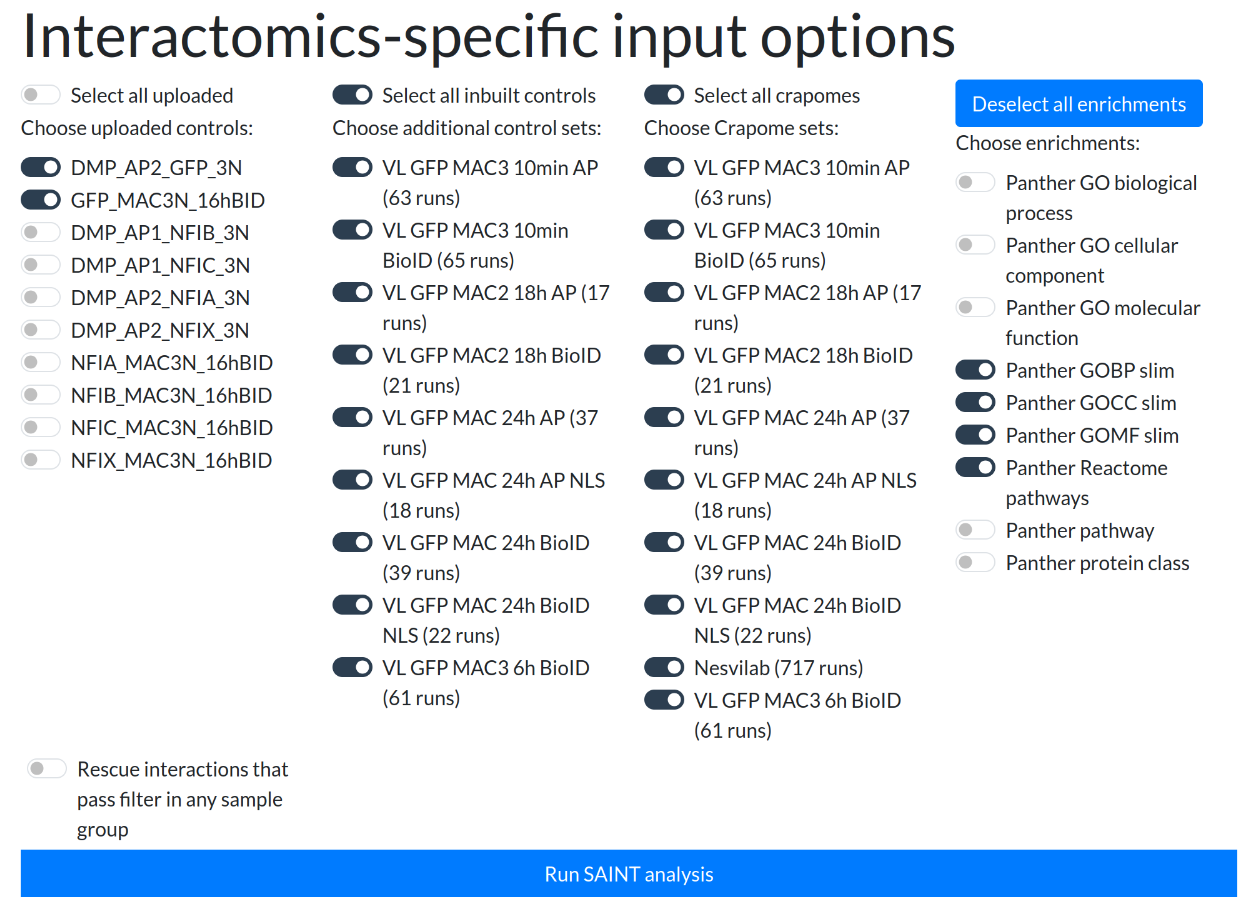the page: In this example we’ve chosen to use GFPs from the sample set as controls, as well as all possible control purification sets and crapome sets, and a few PANTHER enrichments. 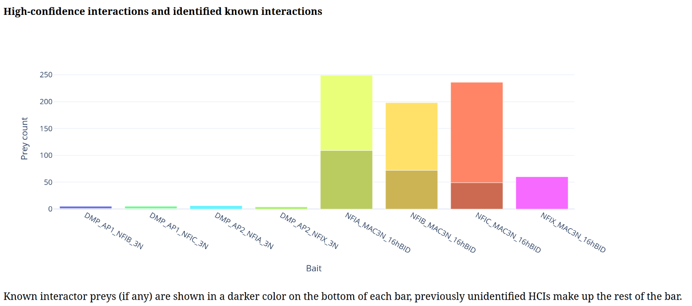After clicking “Run SAINT analysis”, PG will run SAINT, and present another input panel further down the page: 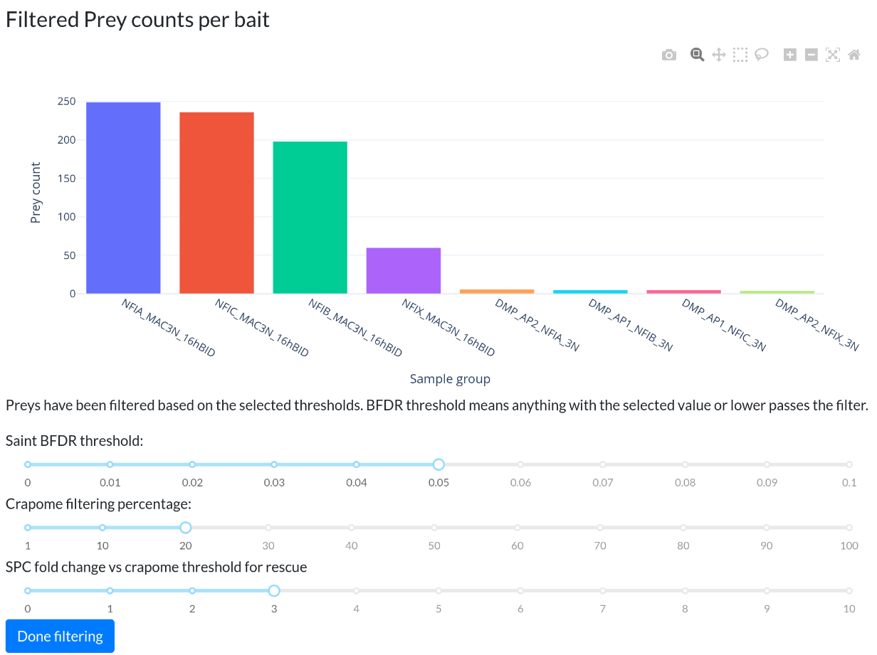Here we see the filtered prey counts with the chosen filters. In this particular dataset, we have some AP-MS purifications together with BioID, so the lower counts on that side are expected. Normally APMS and BioID samples are analyzed in different SAINT runs, but for general QC purposes, this will do.

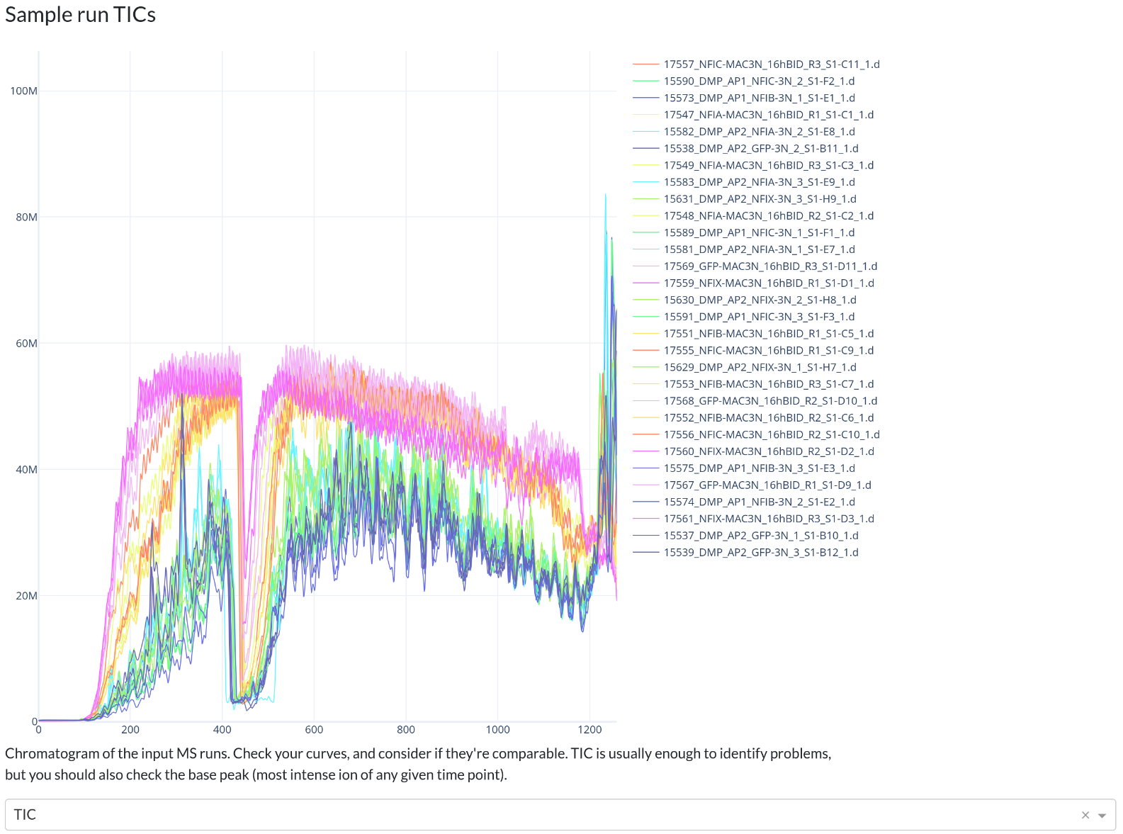
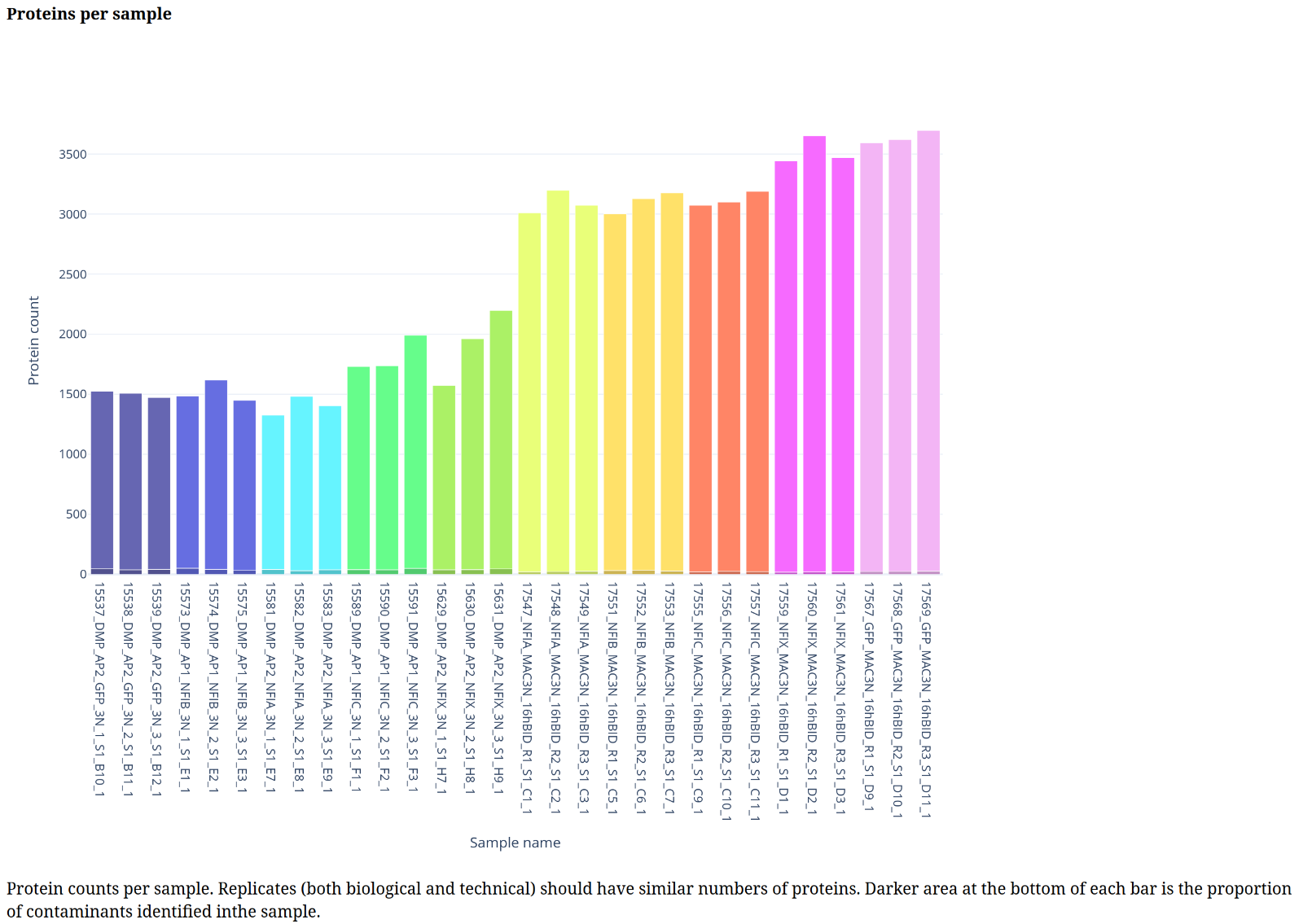
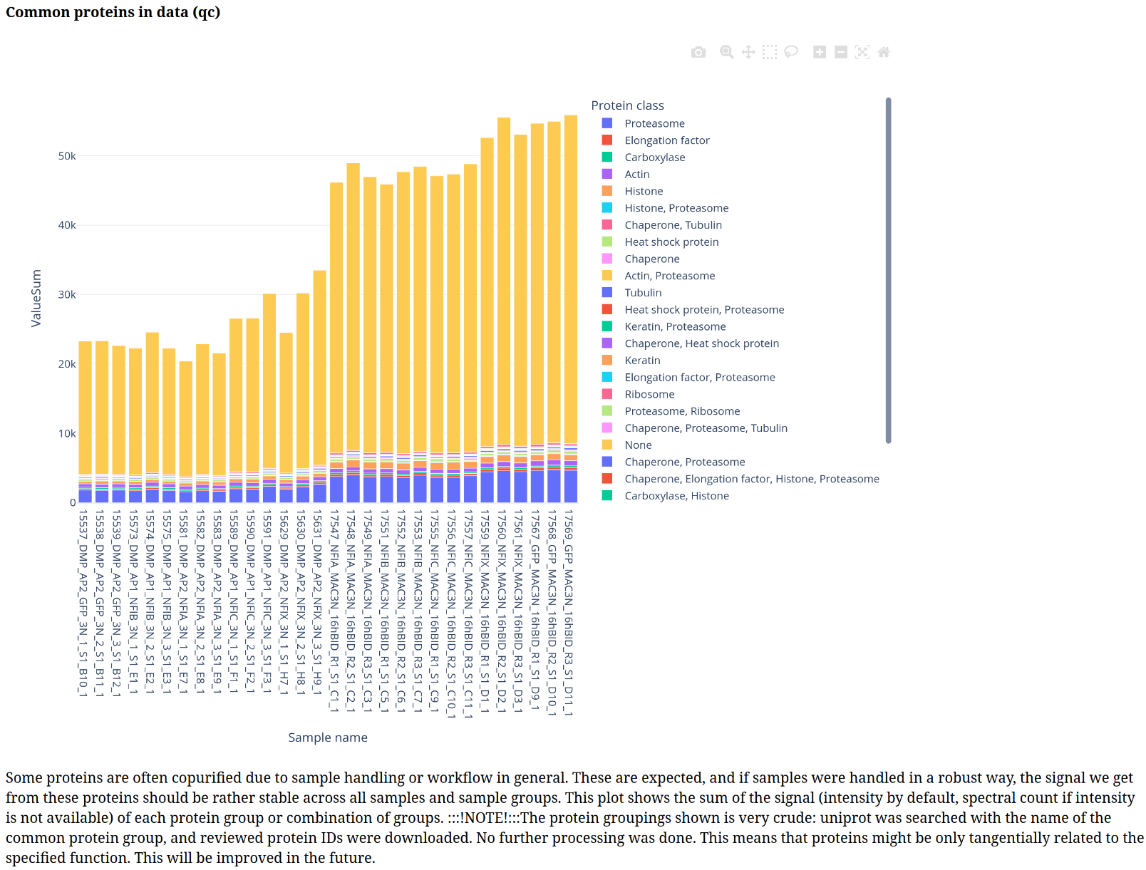
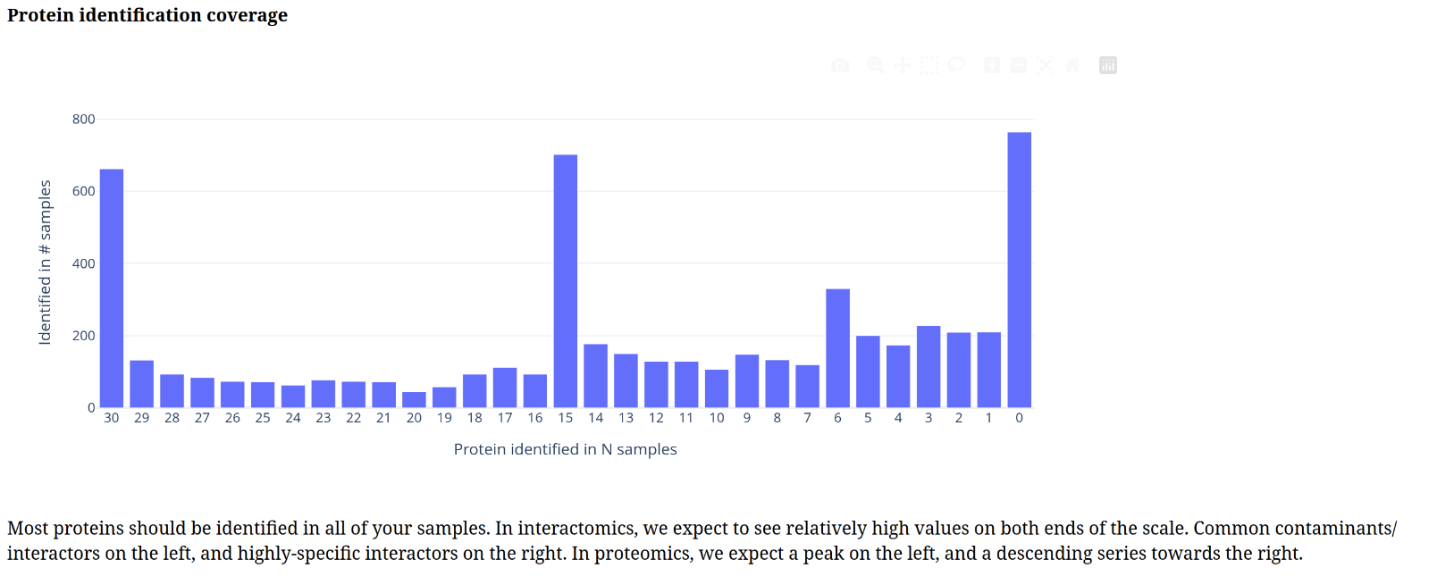
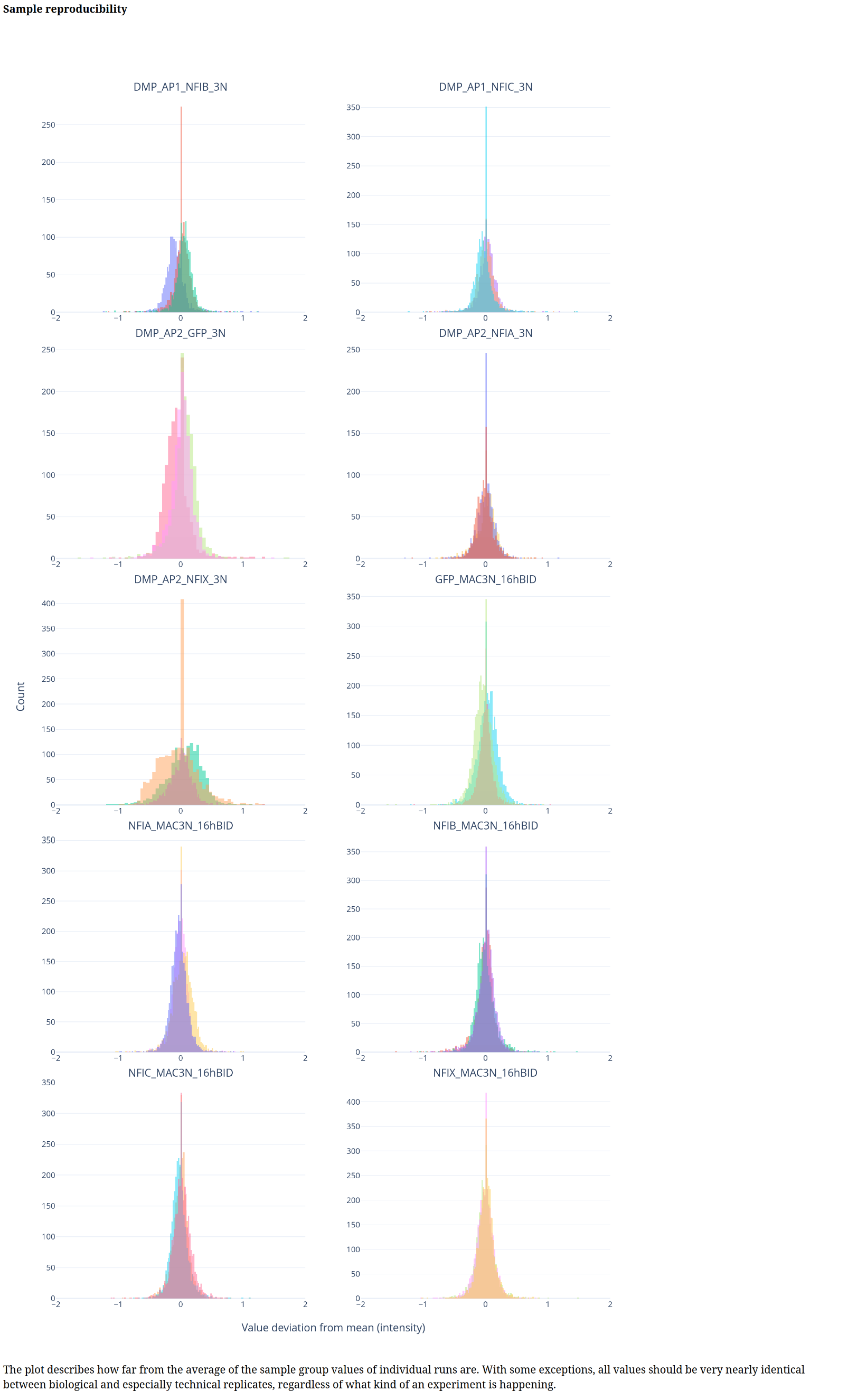
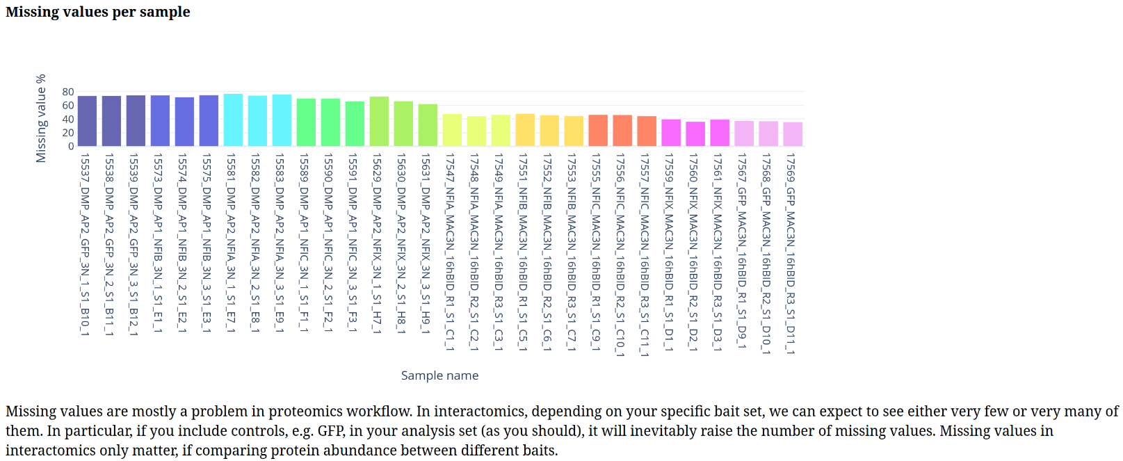
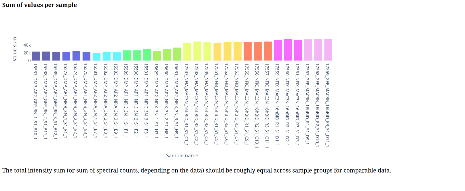
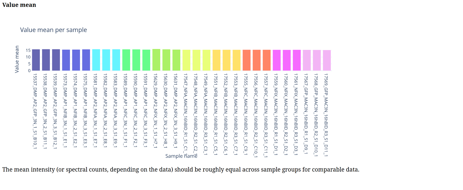
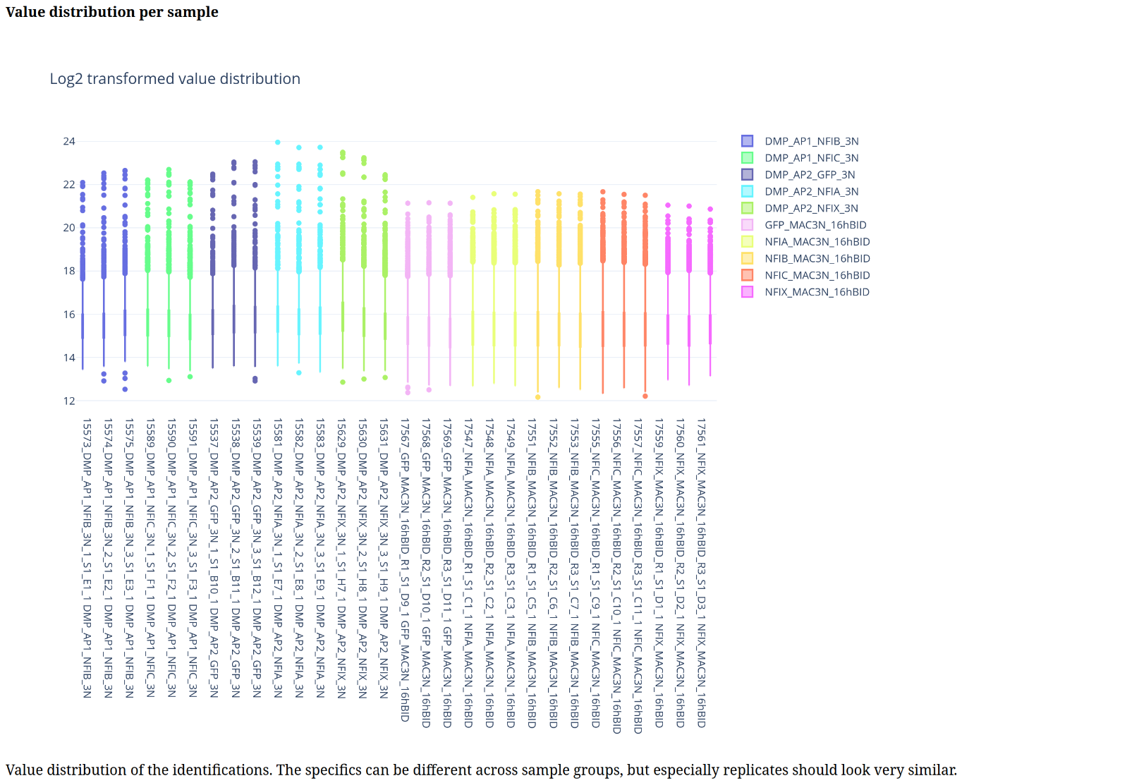
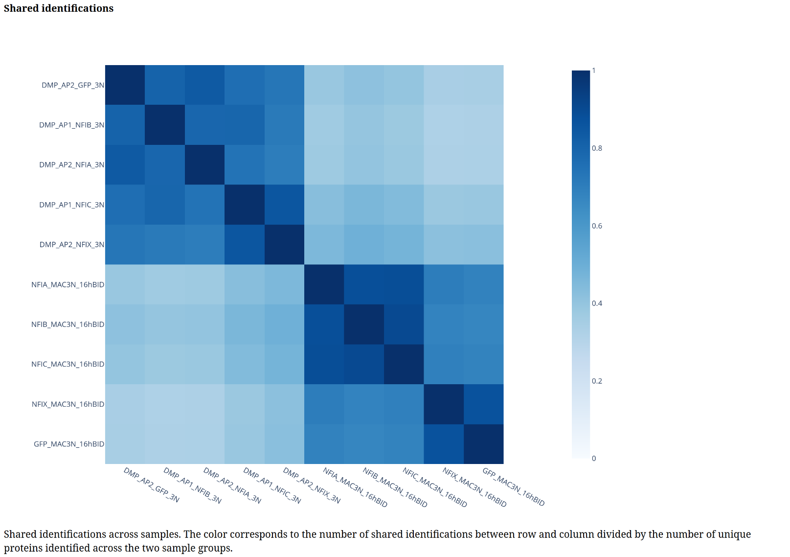
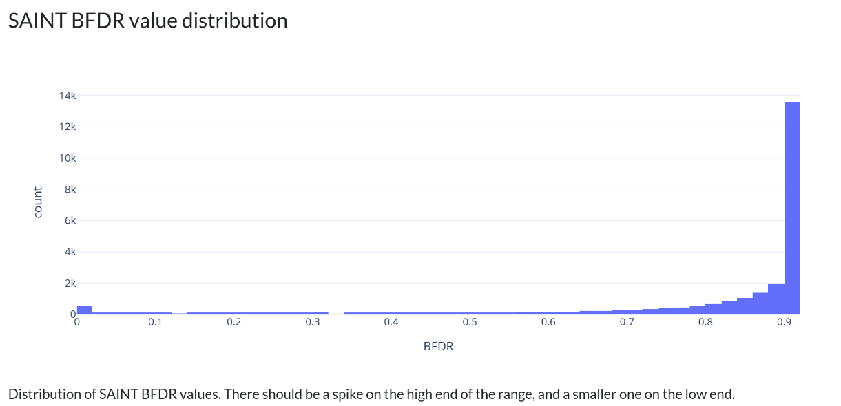
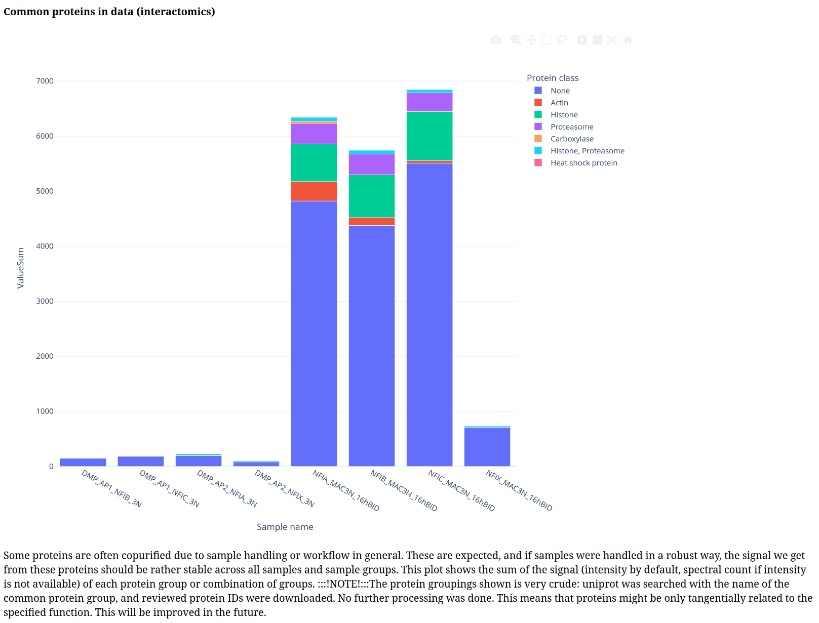
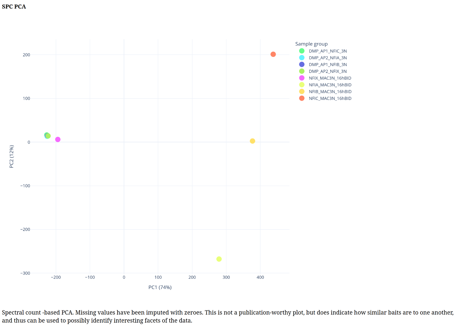
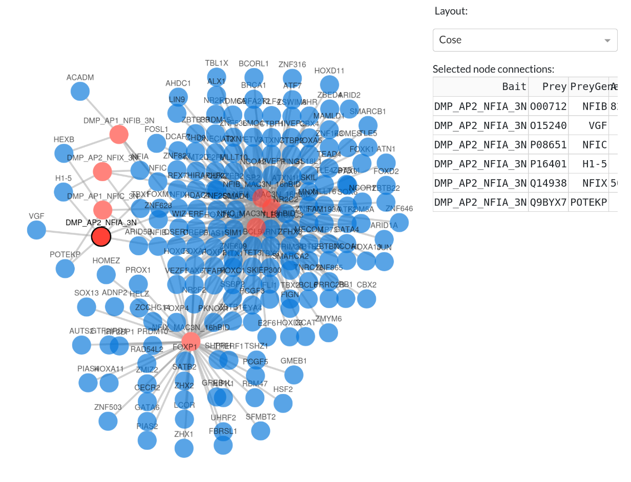
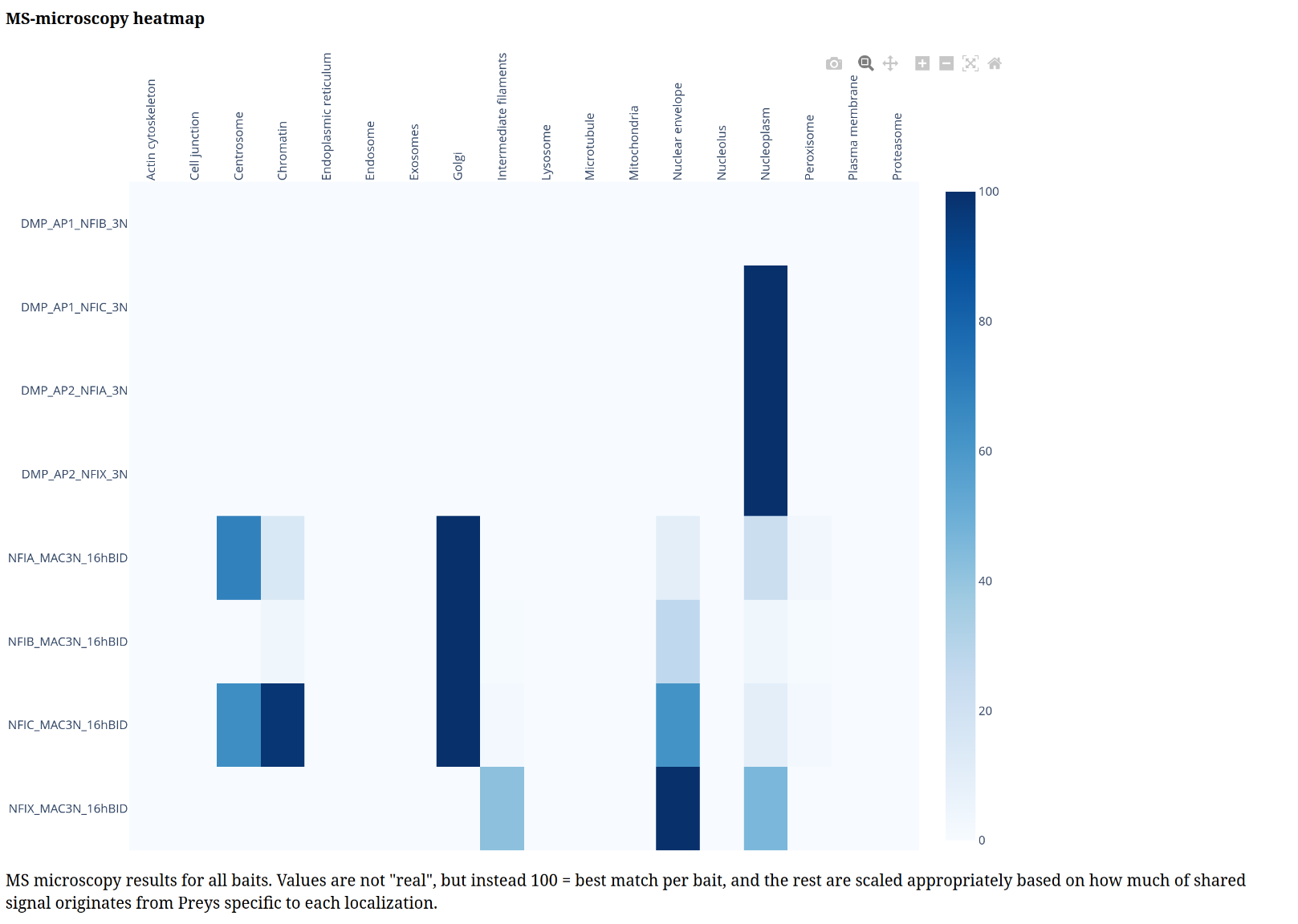
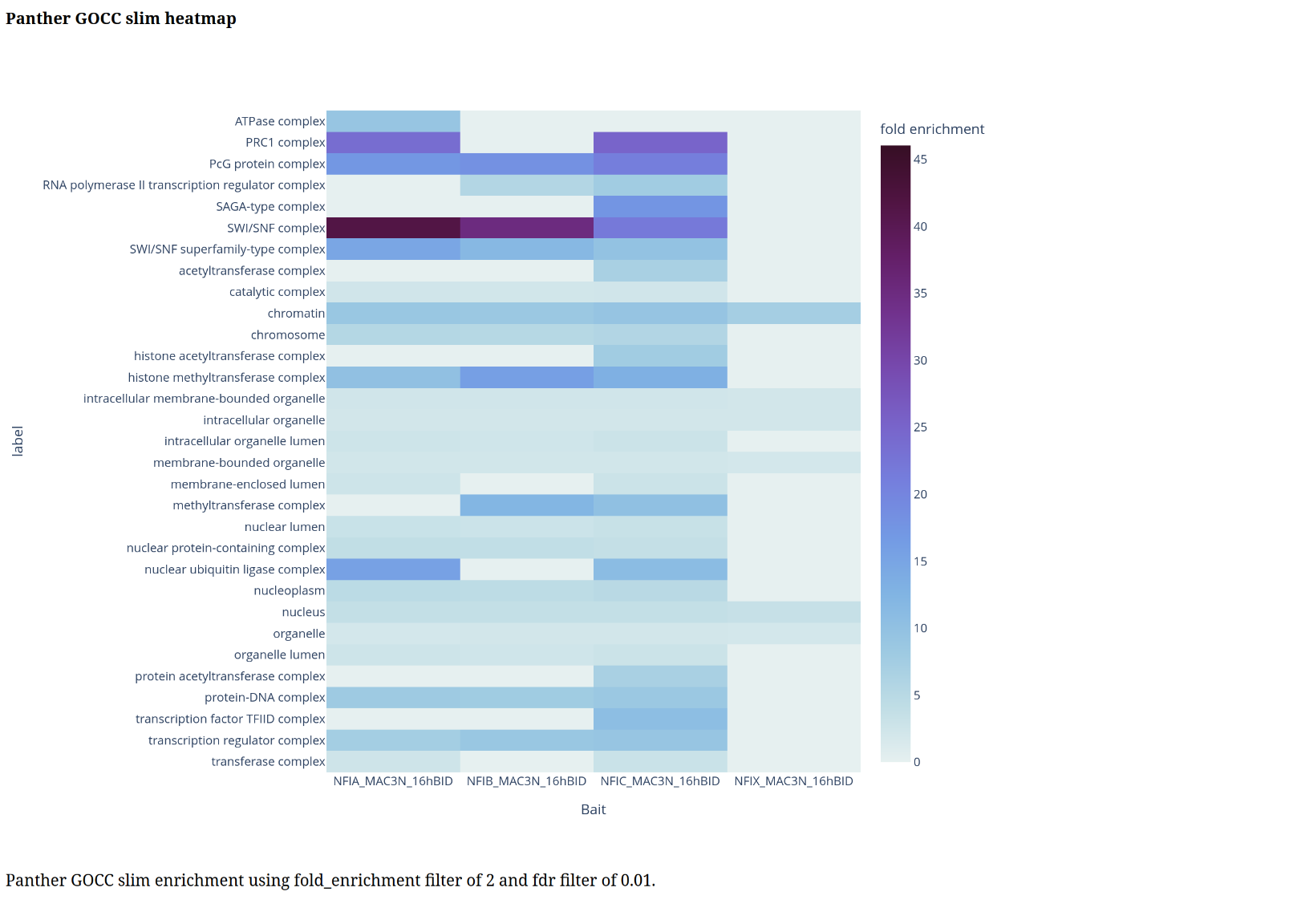
When we’ve chosen the filters we want to use, we can click the “Done filtering” button, and PG will start generating interactomics-specific plots. Below is a gallery of all the generated plots.